Resources

ImageJ

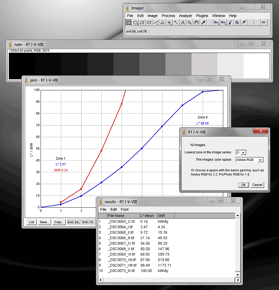
I now measure zone system calibration images using ImageJ, a quirky little utilitarian Java-based program which is also open-source freeware, and can be fully automated with macros and plugins.  I modified the plugin Color Transformer so that images may be converted to L*a*b* for measurement from a number of different color spaces including Adobe RGB and ProPhoto RGB.  With small-gamut images like those of a zone series, it is the gamma that is most important.  I also wrote the BTDZS Zone Ruler macro for ImageJ (link on the Color Transformer page above) that automatically measures all the zone images in a folder, displays their values in spreadsheet form, constructs a zone ruler, and displays a simple plot of the values.

The Beyond the Digital Zone System tool

BTDZS_tool.jsx
BTDZS_tool basic.jsx

The BTDZS tool is what I originally wrote to measure calibration images.  It began as a way to use Photoshop scripting to determine total image noise, then sort of grew out of control.  The important measurements are the mean L* (lightness) value and signal-to-noise ratio.  I have pared the script down to these elements in BTDZS tool basic; it is much simpler to use and probably all you will ever need.

The script works in Photoshop CS2 and CS5 (the versions I have) using Windows XP, 32-bit, and CS5 using Windows 7, 64-bit; I don’t think it will work in prior Photoshop versions.  There are a few differences between how it runs in the versions; the progress bar does not work in CS2, for example, and CS5 uses a color sampler tool that CS2 does not have; but the results are almost identical.

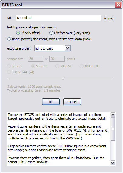
To use the BTDZS tool, start with a series of images of a uniform target, preferably out-of-focus to eliminate any actual image detail.  Append zone numbers to the filenames after an underscore and before the file extension, in the form of IMG_0123_VI.tif for zone VI, and the script will automatically extract them.  (Tip:  when doing multiple batch processes, do this to the RAW files.)  Crop a nice uniform central area; 100-300px square is a convenient size range; but don’t otherwise resize/resample them.  Process them together, then open them all in Photoshop.  Run the script:  File–Scripts–Browse.

Title:  optional; use it to label data with things like the RAW processing settings.  Copy it so you can paste it as the file name when saving the text or .csv file (Photoshop scripting can’t do this automatically).

Mode:  keep the default, batch process L* only, for now.

Exposure order:  batch-processed images are meant to be ordered dark to light.  Choose an exposure order depending on how the images were taken:  dark-to-light, light-to-dark, or middle outward (like V, VI, VII, VIII, IX, X, IV, III, II, I, O), and the script will reorder them for you.  If the images are unrelated, choose “none” and they will be ordered by L* value.  (This option may not work for exposure series because more than one image may have the same lightness value, especially at the high end.)  If the images were not taken in order, or if the order cannot be determined from the file names, you may have to manually rename the files, such as by prepending a two-digit number (01_IMG123, 02_IMG122, 03_IMG121, etc.).  The exposure order setting is saved as an .ini file in your default user folder.

O.K.:  press “o.k.” to process the images; it should take just a few seconds in L*-only mode.  The result includes some basic data in conventional text form, and, more importantly, the entire data output as CSV (comma-separated values).

Save .csv:  press “save .csv,” paste the title that you copied earlier, then save the file.  There are many ways to graph the data; I use a spreadsheet program to open the .csv file (see below).  The spreadsheet data are as follows (the basic ones are highlighted; for now you can ignore the rest):

standard deviation

semideviations

skew

autocorrelation

•  L*mean:  the mean L* (lightness) value of the pixels sampled.

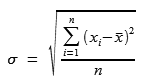
•  luminance noise:  the standard deviation of the ∆L* distances, L* - L*mean.  (It and the total noise are multiplied here by 10 to fit better when graphed with the rest.  The raw values are given later.)

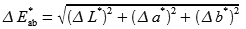
•  total noise:  the standard deviation of the ∆E*ab color distances, square root of ( (∆L*)² + (∆a*)² + (∆b*)² ).  (The conventional ranges of a* and b* are 255, while that of L* is 100; I have scaled a* and b* to ranges of 100 for the purpose of noise measurement, as if the L*a*b* color space were a 100×100×100 cube; otherwise, the total and chroma noise values seem counterintuitively large compared to the luminance noise.  The raw standard deviations are given later.)

•  SNR (signal-to-noise ratio):  L*mean / noise, both luminance and total.

•  L*mean ± L* noise:  sets limits on the meaningful signal above or below the shadow or highlight threshold.  Mostly relevant for the shadows, where it is a kind of noise floor.

•  L*i+½, L*i-½:  the L*mean halfway between the L*mean of the current zone and either the next higher or lower zone; the limits of “the whole zone” referred to earlier.  If the images are not a stepped series, this and the next two measurements have no significance.

•  zone L*:  the L* interval that an image represents in relation to the ones before and after it; the width of “the whole zone”; L*i+½ - L*i-½.

•  zone SNR:  SNR based on the interval, not total, signal; zone L* / noise.

•  a*mean, b*mean:  the mean a* and b* value of the pixels sampled.

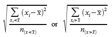
•  L* positive and negative noise:  the semideviations (standard deviation of values in one direction only) of the ∆L* distances.  I thought they might be useful in relation to the noise floor or highlight threshold, but so far I haven’t found them to be.

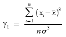
•  skew:  accompanies the semideviations; a measure of how one-sided the distribution is.  Tends to depart from zero near the highlight and shadow thresholds.

•  chroma noise:  the standard deviation of the ∆ab distances, square root of ( (∆a*)² + (∆b*)² ), scaled to ranges of 100 like the total noise above.  Chroma and luminance noise constitute the total noise.

•  chroma and total s.d.:  the raw, unscaled standard deviations.

•  L*min, L*max:  the minimum and maximum L* values of the pixels sampled; 0 or 100 usually means that the values are clipped.

•  SNR (dB):  SNR in decibels, 20 * log10 (SNR).

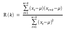
•  correlograms:  histograms of the autocorrelation of pixel L* values at increasing distances, in number of pixels, from each other; a measure of noise quality.  High autocorrelation values indicate a nonrandom spatial distribution, or clumping, of the image noise; negative values may indicate halos.

•  pixels, pairs:  the number of pixels and pixel pairs used to generate the correlograms.

•  area:  the absolute value of the area under each correlogram.  Smaller value = more random distribution.

Save text:  the text part of the output also includes the following:

•  n:  the number of pixels sampled.

•  noise, SNR:  in color modes, displayed as pairs of values, L* and total.

•  mean color:  the mean L*, a*, and b* of the pixels sampled.

•  color (L*, a*, b*) and distance (∆E*ab):  in single-document mode, the L*a*b* color, and distance from the mean, of each pixel sampled.

The other modes:  the L*-only mode uses pixel data from the L* channel histogram, which is very fast.  The color modes must sample each pixel individually, which is a slow process, but includes the color data (such as total and chroma noise, the data that are blank in L*-only mode) in the results.  Batch process L*a*b* color mode samples the data from each open image, like L*-only does.  The single (active) document mode includes the color (L*, a*, b*) and distance (∆E*ab) of each pixel sampled.

Sample size:  in color modes, the sample size is determined by the values in the sample size fields.  The size may be increased from the default 50 × 20 at the expense of longer processing times (about 38 seconds per 1000 pixels on my 2.79 GHz machine).  Adjust the size by typing in new values, clicking the radio buttons, or moving the slider.  The default sample width is 50 pixels to allow for an adequate amount of data for the autocorrelation measurements, which are taken in the horizontal dimension.  The sample is centered in the image.  In L*-only mode, the entire image is sampled (which may start to slow down the script if very large images are used).

Cancel:  interrupts the script if it is taking too long.

Unlike the Photoshop histogram statistics, the BTDZS tool uses the absolute color distance to measure noise, rather than separate measurements of the color channels, so the standard deviation of a solid color is always zero.  The CIE76 color distance metric (∆E*ab, the Euclidean L*a*b* distance) is used rather than CIE94 (the weighted L*C*h distance) because the latter is unreliable when measuring colors of low chroma.

Note:  when saving the text or .csv, files with the same name will be overwritten without warning.  Unless the file is already open by another application, in which case it will not be saved, again without warning.  It’s a Photoshop scripting thing.

Spreadsheet programs

I use Microsoft Excel 2000 because I happen to have it.  It is a great program overall, but if you are interested, I recommend looking for a version prior to the major revision of 2007 (search “hate Office 2007” for details), or waiting until Microsoft changes it back to the way it was.

A great freeware program is Calc from LibreOffice.org (formerly OpenOffice.org).  It has most of the functionality that Excel has; one annoying feature is that there is no option to generate a chart on a separate sheet, you have to manually cut/paste/size/position it yourself.  Also, it is a little more complicated to change the source data of an existing chart.  But the graphs themselves look good.  The download is large and includes the entire suite of programs (word processor, database, etc.); you can choose to install only the components you want.  I used Math to generate the equations above.

Either of the above programs will open the .csv files generated by the BTDZS tool and automatically format them as a spreadsheet; then all you have to do is select data and create a chart.  There are many other graphing programs, some of which will import data from a .csv file; search “csv graph” if you want to look around.

Sample spreadsheet

Here is a sample spreadsheet for the BTDZS tool that illustrates how the charts are made.

Raw editors

For zone system calibration, I recommend RawTherapee.  Version 4.1, released in May 2014, is a substantial improvement over the previous versions, and in my opinion it is Adobe’s only serious competitor.  It can do some pretty good general photo editing as well.

Then there are Photoshop, Photoshop Elements, and Lightroom, which all use Adobe Camera Raw as their raw converter.  For zone system calibration, use the Process 2010 controls, as Process 2012 is adaptive and does not provide a fixed baseline.

Others include Capture One by Phase One; Photo Ninja; AfterShot Pro (formerly called Bibble); Silkypix; UFRaw, on its own or as a Gimp plugin; and darktable.  I have not found any other raw converter to be particularly useful for zone system calibration.

PhotoLine

PhotoLine is Photoshop’s main competitor.  Unfortunately, the documentation is not always the best, and some of the menu items are inexplicably in German.  But it has some unique features, such as saturation and L*a*b* curves in an RGB image, and adjustment layers for adjustment layers.  It also uses Photoshop plugins.  Best of all, you can buy a permanent license for only €59!

Other downloads

Printer targets, RGB and L* increments; and standard texture target.  Thumbnails are links to the .tif images.

It is important to print the texture target on matte paper that has no optical brighteners.

ZoneRuler.jsx – Photoshop script that creates a zone ruler from the open images.  New and improved 6/12/2012, it now adds black and white bars at the bottom and top for reference.