|
|
Going to Extremes
As previously mentioned, I consider the output of a RAW processor to be raw material, so to speak, and prefer to create the final image with advanced tools in an editor such as Photoshop. (Not that RawTherapee doesn’t have advanced tools of its own . . . .) For example, the linear output of RawTherapee, without applying a contrast curve of any kind, looks pretty dull and flat to the eye. But a contrast S-curve is only one way to alter the contrast and dynamic range of an image. Two other ways are high-radius low-amount unsharp masking and histogram equalization. The former can easily blow whites and block blacks if taken too far, especially if the overall image contrast is already high; but the results are often more interesting than the application of a simple S-curve.
So why not leave out the S-curve during raw processing, and leave as much head and foot room as possible at the highlight and shadow thresholds, to facilitate future processing? One way to do this is to consider the shadow and highlight threshold values, 2 and 98 in our case, as just a minimum and maximum, respectively. Zero all the exposure tab controls, and set all the curves to Linear. Leave the Avoid color shift box unchecked to prevent a paradoxical increase in the shadows above a certain Black level, among other things. Then lower Exposure Compensation as far as possible while keeping a blown white, such as zone XI, at 100. Raise the Black control to lower the black limit, zone -I in the previous examples, to as close to 0 as possible. Now adjust the Lightness control to put the desired middle gray zone on 50. The highest zone with a value less than or equal to 98 is the highlight threshold. The shadow threshold is the zone above the black limit. Its value should be at least 2; move the black limit up one zone if it is not. Analyze the results with ImageJ to make sure that the shadow threshold signal-to-noise ratio is acceptable. (See the RawTherapee page, if you haven’t already, for an explanation of the above.)
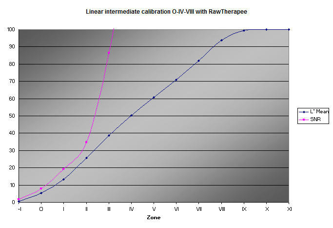
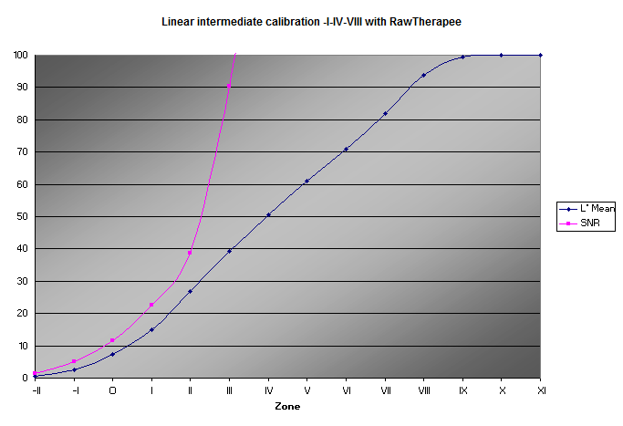
The first graph below is the result of placing zone O on the shadow threshold, and zone IV on middle gray. The zone O value is 5.2, well above the minimum, and the SNR when calibrated this way is an ample 7.86. The second graph is the result of moving the shadow threshold down to zone -I; its value is now 2.6, the SNR is 5.17, and the zone VIII value is 93.7. These values indicate that, during exposure, useful shadow information may extend all the way down to zone -I. Note how straight the L* curves are:
|
|
|
|
Note that in the series above, there are between 12 and 13 zones, not 10! But they are not all equally useful, and we may lose a few at the extremes when we manipulate the image as illustrated below. The point is that we have plenty of room to work in.

|
||||||||||||
| -II | -I | O | I | II | III | IV | V | VI | VII | VIII | IX | X |
In practice, one may choose to just leave the Black setting at zero, and pay attention to shadow values and noise in the final image, adjusting if necessary. The only fixed nonzero value in this case is Exposure Compensation, chosen based on the calibration above. The Lightness control may be adjusted to taste. (One may still use the camera’s .dcp and lens profiles, white balance, chromatic abberation, and other color controls such as the CC curve as desired.) Tip: apply a contrast curve to reality-check the Lightness and color settings, then remove it before processing.
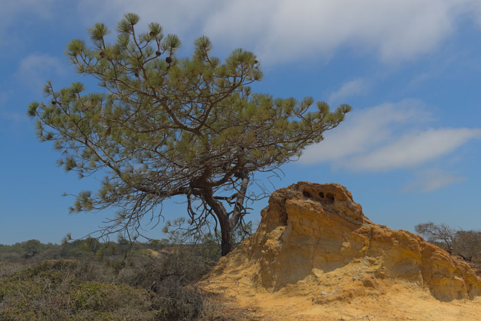
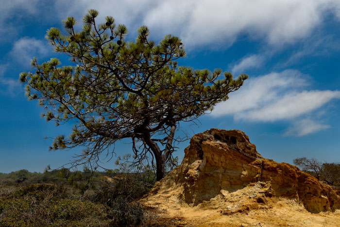
The resulting long-scale image, such as the first one below, may not be much to look at. Think of it as an intermediate, such as photographic negative, or a transparency that is intended to be printed, and not the final product. The second image is more like a final product, made from the first with global and local applications of high-radius low-amount unsharp masking, as well as other adjustments (including curves).